Two Methods for Improving Nearest Neighbor Searching in Motion Matching

A new way to next generation of animation

Posted Jul 23, 2024 Updated Feb 20, 2025

6 min read

In the last previous blog, we talk about the basic idea of Motion Matching. And the process of original Motion Matching can be illustrated as follows.

design dance cards
Motion capture and create dataset
find the motion with smallest distance
jump to the motion

However, there are still some problems when implementing Motion Matching.

brute-force search method is not efficient
discontinuity when jumping to the new motion
the dataset incurs large memory overhead

In this article, I want introduce two methods improving the NN searching efficiency in Motion Matching.

KD-tree
voxel-based method

KD-tree

KD-tree is extension of binary search tree in higher dimension.

As we all kown, the time complexity is $O(N)$ when we use brute-force search. It could be disaster when the size of the samples is too large.

And the BST can improve the performance to $O(logN)$ by structured store the data like this.

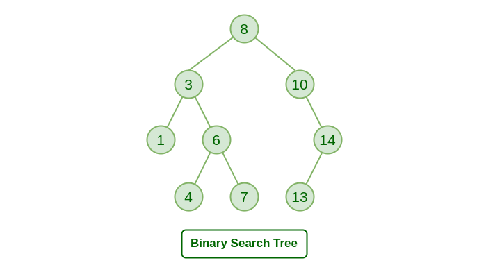
all values of nodes in left subtree are smaller than the value of the root.
all values of nodes in right subtree are larger than the value of the root.
the left and right subtrees are both binary search tree.

it seems like we put all the nodes on a number line, and divide them into two part by finding the median.

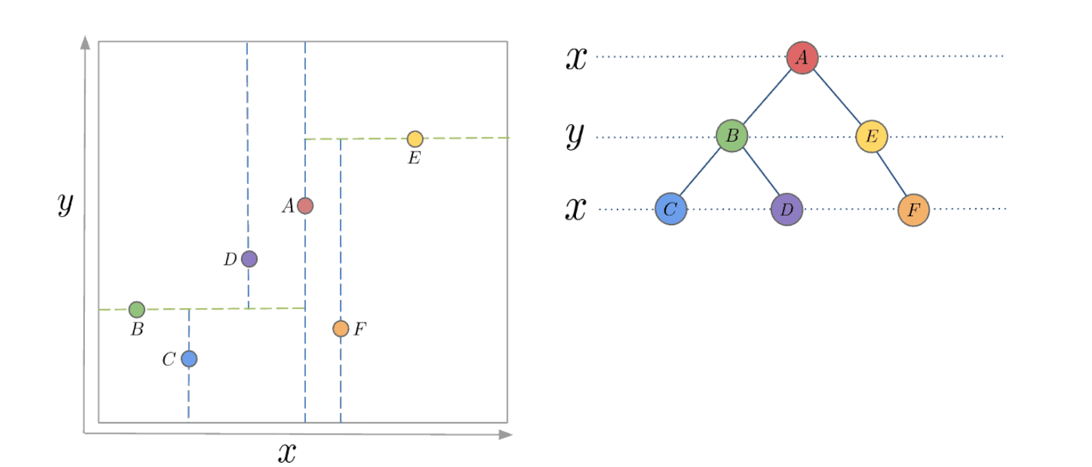
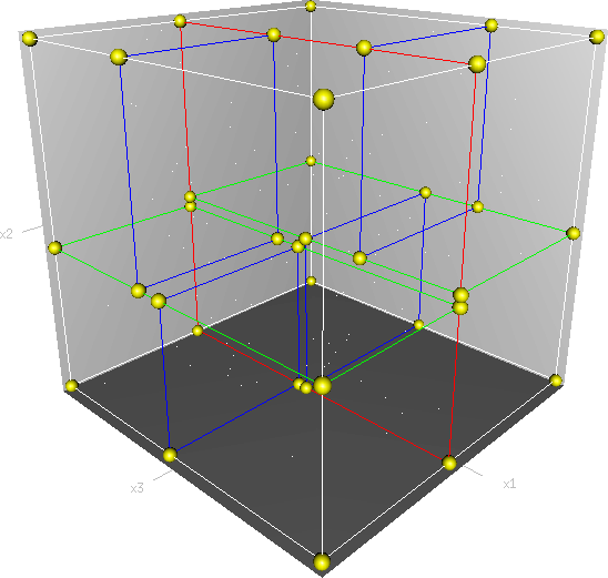
KD-tree uses the same method, every non-leaf node in the tree acts as a hyperplane, dividing the space into two partitions. in 3 dimension and 2 dimension scenarioes, it still can be illustrated.

There are different strategies for choosing an axis when dividing, but the most common one would be to cycle through each of the K dimensions repeatedly and select a midpoint along it to divide the space.

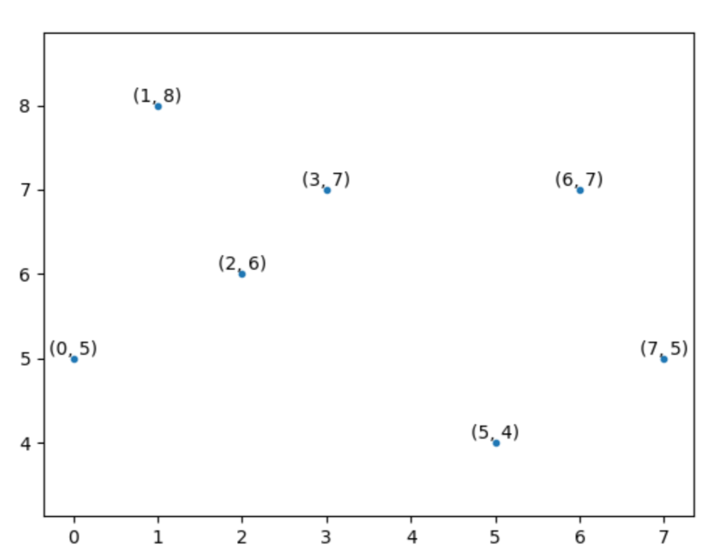
kd-tree construction algorithm is shown in the image below:

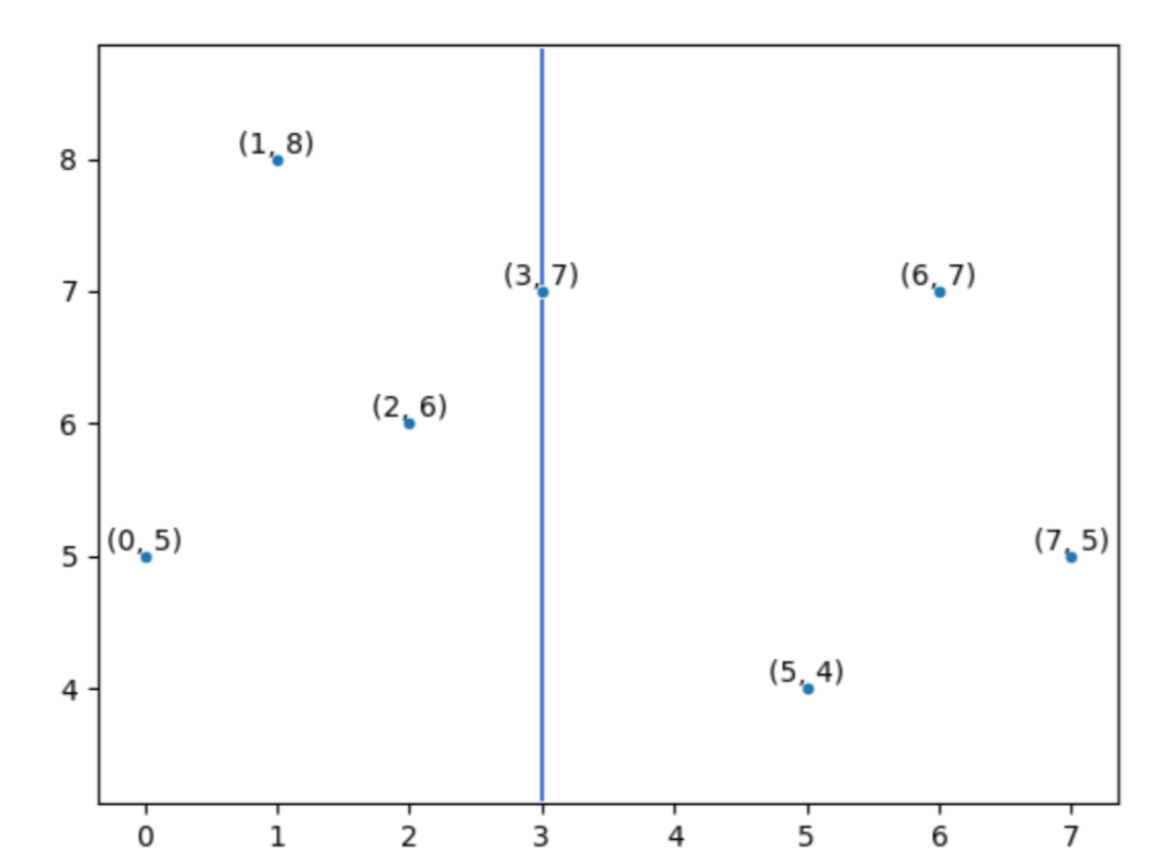
Taking the case of 2 dimension as an example, some 2d data is shown as the figure below:

X axis could be the first dimension or attribute for partition. Find the median on x axis, and then divide the 2d plane into two parts.

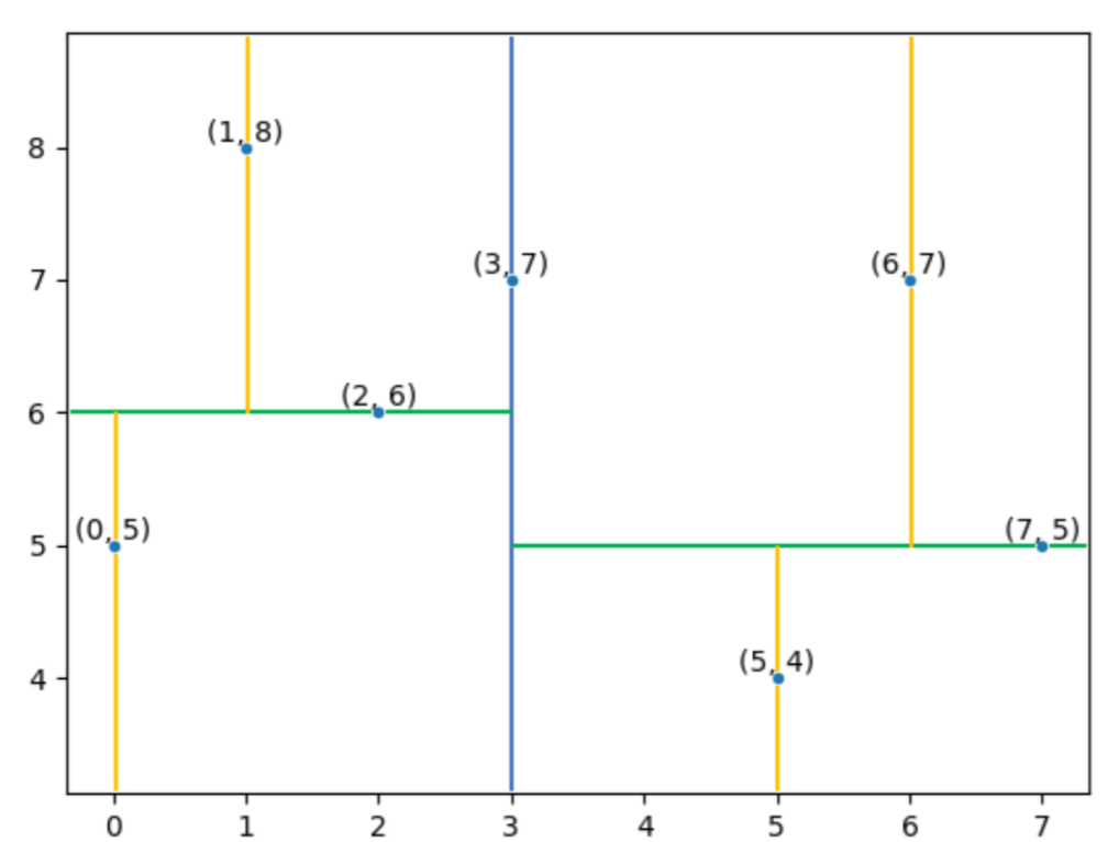
Y axis could be the next attribute for new partition. Find the median and divide.

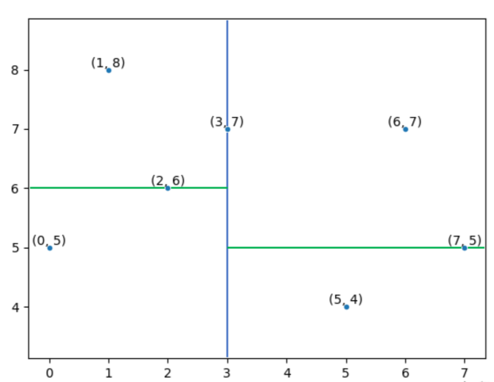
And then repeat the same thing

The foregoing section is about the construction of kd tree. Next, I will discuss the nearest neighbor search using kd-trees.

Users input a query point to find the nearest neighbor. The algorithm begins by determining which hyperspace the query point belongs to. It records all the nodes traversed during this process in a stack. After this initial step, the algorithm calculates the distance between the query point and the leaf node, which is denoted as the current best distance.

However, there may be other nodes stored in the stack that have a lower distance to the query point. To find these, the algorithm recursively calculates the distance between the query point and each node in the stack. Whenever a node with a lower distance is encountered, the current best distance is updated accordingly.

This recursive traversal of the nodes in the stack allows the algorithm to efficiently find the nearest neighbor to the query point, by continuously refining the current best distance as better candidates are discovered. The use of the stack ensures that the algorithm keeps track of the relevant nodes visited during the search process.

If you wanna know more, please refer to the link at the end of this blog.

voxel based lookup table

Voxel-based methods are another efficient approach for searching for nearest neighbors in a dataset. Similar to KD-trees, they improve efficiency by structuring the stored data. The key idea is to categorize samples with similar feature vectors into individual voxels (discrete 3D grid cells).

In Kinamatica, a system first proposed by the Unity team at GDC 2018, Michael Buettner enhanced the implementation of motion matching using a voxel-based approach.

Notations

Some notations for further illustrating the methods:

A root transform $T$ representing the coordinates and orientation of the character. $T = (p,q)$, where $p$ and $q$ represents coordinates and orientation respectively. T is called the position of the character.

A set of primary joint position $J = {J_{i}; i = 1,2,…,M}$, where $J_i = (x_i , y_i , z_i)$, To optimize run time complexity, all joint positions are expressed relative to the root transform $T$.And further denote $\mathcal{J}$ the set of all possible joint value. the value of joints $J$ w.r.t. some $T$ is called its pose.

The pair position-pose id called its state $s = (T,J)$.

Trajectories of the character in the game world are represented by sequences of root transforms that span over the immediate past and future:

\[H = (T^{-\tau},T^{-\tau+1},...,T^{0},...,T^{\tau-1},T^{\tau})\]

where $T^0T$ is the current position , and ${\tau}$ is the planning horizon i.e. one second.

Animation data comes as a set of clips $\mathcal{C} = { C_{i} ; i = 0,1,…,N }$. Each clip is a series of character states: $C_i = {(T_{i}^{k},J_{i}^{k}), k=0,1,…,L_{i}}$.

All the animation clip segments selected from the mocap data are stored in a large matrix $D$, the database.

Method

First step is to identify the highest variance joints in the database $D$.

The next step is to discretized the space of values for this joint in a fixed number of bins. This is aim at create a voxelized representation.

In the final step, the voxels are filled with references to the poses in D using the following process:

for every pose $J$ in the MoCap dataset $D$, look-up the value of the highest-variance joint into the voxelization. So, we can get a cell $c$ where $J$ projects to.
use a pose-comparison function $f$ to tell other pose $J^{\prime}$ in the dataset is successor of this pose $J$ or not. If positive, add this pose $J^{\prime}$ into cell $c$

By doing this, we can get the structured data $\mathcal{V}$

One thing remained is the pose-comparison function.

The natural successor of pose $A$ is denoted as $A^{+}$, similarly, the predecessor of the pose $B$ is dentoed as $B^{-}$.

To make the comparison specialized and more efficient, only part of joints are selected according to different task.

\[\bar{J} \subset J\]

For instance, for an application to standard bipedal locomotion, $\bar{J}$ contains the joints of the left and right foot as well as the neck joint.

And then perform the following testing:

For every $j \in \bar{J}$, to test

\[\|j_{A^+} - j_{B}\| < \sigma (v_{AA^{+}}(j))\]

where $\sigma(x) = ax + b$, and $v$ represents velosity. Because when the object is at a high speed, it can afford larger difference between current pose and successor.

Another test should be done between these two vectors:$j_{A^+} - j_{A}$ and $j_{B}-j_{A}$. The test passes if the direction of these two vectors do not differ by more than 90 degrees. This test focuses on the speed of the joint instead of its position.

The last test compares the norms of the joint speed in pose $A^+$ and $B$.

Define

\[v_{B^{-}B}(j) = \|j_B - j_B^-\|\]

Then test passes if

\[\|v_{AA^{+}}(j)-v_{B^{-}B}(j)\|< \sigma^{\prime}(v_{A}(j))\]

Again, $ \sigma^{\prime}(x) = a^{\prime}x + b^{\prime}$

These three tests are all about the pose-comparison function.